1. Introduction

The fine-tuning argument is regarded as one of the strongest arguments for the existence of God in contemporary philosophy of religion, the cutting-edge in the long tradition of design arguments for God.

In his article in the Blackwell Companion to Natural Theology, Robin Collins states the core fine-tuning argument thus (edited here only to expand Collins’ acronyms): (p. 6)

(1) Given the fine-tuning evidence, a life-permitting universe (LPU) is very, very epistemically unlikely under Naturalism and a single universe (NSU): that is, P(LPU|NSU & k′) << 1, where k′ represents some appropriately chosen background information, and << represents much, much less than (thus making P(LPU|NSU & k′) close to zero).
(2) Given the fine-tuning evidence, LPU is not unlikely under Theism (T): that is, ~P(LPU|T & k′) << 1.
(3) T was advocated prior to the fine-tuning evidence (and has independent
motivation).
(4) Therefore, by the restricted version of the Likelihood Principle, LPU strongly supports T over NSU

In this article, I will examine the argument Collins uses to defend (1), and argue that his argument makes a faulty assumption.

2. Arguing for (1)

The core support for (1) is of course the fine-tuning evidence. A discussion of such evidence is far beyond the scope of this article, so on this topic I will refer the reader to the discussion in Collins’ article and to the excellent and detailed discussion by astronomer Luke Barnes.

The gist of this evidence is that in order for life to be possible in our universe, given our best understanding of physics, the fundamental constants of our universe must lie within extremely narrow intervals, relative to the range of values that a priori they might have taken.

2.1. The Principle of Indifference

How do you get from “narrow intervals” to “low probability”? To do this, you must assume some probability distribution on the possible values the fundamental constants could have taken. Towards this, Collins introduces the following principle: (p. 33)

According to the restricted Principle of Indifference, when we have no reason to prefer any one value of a variable p over another in some range R, we should assign equal epistemic probabilities to equal ranges of p that are in R, given that p constitutes a “natural variable.” A variable is defined as “natural” if it occurs within the simplest formulation of the relevant area of physics.

[…]

Since the constants of physics used in the fine-tuning argument typically occur within the simplest formulation of the relevant physics, the constants themselves are natural variables. Thus, the restricted Principle of Indifference entails that we should assign epistemic probability in proportion to the width of the range of the constant we are considering. We shall use this fact in Section 5.1 to derive the claim that P(Lpc|NSU & k′) << 1, where Lpc is the claim that the value for some fine-tuned constant C falls within the life permitting range.

In other words, Collins argues that we have no reason to think any values of the fundamental constants are a priori any more likely than any other, and so we should assume a uniform distribution on the possible values of the constants. He then later argues for (1) as follows: (p. 51)

(i) Let C be a constant that is fine-tuned, with C occurring in the simplest current formulation of the laws of physics. Then, by the definition of fine-tuning, Wr/WR << 1, where Wr is the width of the life-permitting range of C, and WR is the width of the
comparison range, which we argued was equal to the width of the Epistemically Illuminated range [the range of values for which physics tells us whether those values are life permitting].
(ii) Since NSU and k′ give us no reason to think that the constant will be in one part of the EI range instead of any other of equal width, and k′ contains the information that it is somewhere in the EI range, it follows from the restricted Principle of Indifference that P(Lpc|NSU & k′) = Wr/WR, which implies that P(Lpc|NSU & k′) << 1.

This assumption of a uniform distribution will be our target in this article. However, before we delve into that, it will be good to briefly review the virtues of the Principle of Indifference. Given no information, a uniform distribution is the most natural to assume, precisely because it does not arbitrarily favour any particular outcome over any other for no good reason. Furthermore, a uniform distribution is what you get when you average over all distributions that might govern the outcome.

This latter perspective is going to be important in what follows, so let us be explicit about it. We will suppose that our fine-tuned constant $C$ is randomly sampled from an unknown distribution $\mathcal{D}$ . Then if we had no information regarding $\mathcal{D}$ , we would have to assume it is uniform, as Collins argues.

3. Things we know about the distribution

However, this state of total ignorance about $\mathcal{D}$ isn’t really the situation we find ourselves in, and this introduces a hiccup in Collins’ argument.

3.1. Normality

If we are supposing Naturalism, we must suppose that the universe and its constants came about by some natural process. But here’s the thing about natural processes: they don’t tend to give rise to uniform distributions. Consider the distribution of human height (taken from https://ourworldindata.org/human-height):

distribution-1

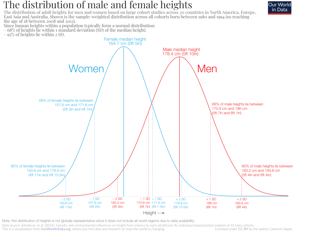
What this is not is a uniform distribution. Instead, it resembles far more a normal distribution. And height is not a cherry-picked example; normal distributions are extremely prevalent among naturally occurring quantities.

Given this, it is reasonable a priori to suppose that $\mathcal{D}=\mathcal{N}(\mu,\sigma^2)$ , a normal distribution with unknown mean $\mu$ and standard deviation $\sigma$ .

3.2. An estimate for the mean

At first, this assumption of normality seems to achieve very little. We have no clue what $\mu$ might be, so by the Principle of Indifference we must suppose $\mu$ is uniformly distributed. But then our best guess for $\mathcal{D}$ is an average of normal distributions over all possible means, which is once again a uniform distribution.

But there is a flaw in this reasoning: we are not in a situation where the Principle of Indifference applies. We do not have no information at all about the distribution governing our universe: we have a data point. The actual value for $C$ in this universe is a value sampled from $\mathcal{D}$ , and therefore is on average close to the mean of $\mathcal{D}$ .

More formally, given the data that $C$ takes a given value, it is standard to infer that $\mu$ takes whatever value that would make it most likely we would observe that data (this is called the maximum a posteriori estimator or MAP). But the data is most likely when it is exactly average, so we should infer that $\mu$ equals the value for $C$ that we observe.

(Bayesians reading this might not approve of using MAP here, in which case we can easily show, and indeed it is visualised in the below figure, that if $\mu$ has a uniform prior distribution, and we observe that $C = c$ , then we have posterior distribution for the mean $\mu \sim \mathcal{N}(c,\sigma^2)$ .)

This might be a bit abstract, so lets give an example. Below is a bunch of experiments of random points on the unit circle with argument normally distributed with uniformly random mean (and standard deviation of pi/10) . The red dot indicates the mean value. The orange dot indicates the very first point sampled for each circle. circles normal no axes2 Notice how the orange dot is a pretty decent estimate for the mean in most of the experiments.

4. Conclusion

So, what is the upshot of all this? The argument above aims to show the following:

Given Naturalism, we should infer that the possible values for the constants of the universe are normally distributed with mean the values we observe them as taking.

Given this, it is then no longer clear that on Naturalism it is unlikely that a given constant will fall in the life-permitting range. Whether this is true or not will depend on the width of the life-permitting region relative to the unknown standard deviation $\sigma$ . If $\sigma$ is low then it is quite likely a universe will permit life, whilst as $\sigma\rightarrow\infty$ we return to the case of a uniform distribution. But this then presents a roadblock for the proponent of the fine-tuning argument: by what principle do they propose to argue that $\sigma$ is large rather than small?

These difficulties may not be all too insurmountable. This may not be a rebuttal to the fine-tuning argument, but it does at least present an issue with how it is usually formulated, and seems to me to show that arguments based on a direct application of the Principle of Indifference rest on shaky ground.

Post-script

A reasonable objection here is that this argument only considers a single fine-tuned parameter. We made this simplification because Collins does, and because it makes the maths simpler, but what happens if we consider more parameters? The argument still seems to remain intact!

Let us write it as a syllogism:

If naturalism is true, the vector $\mathbf{X}$ of parameters of a random universe obeys the multivariate normal distribution $\mathbf{X} \sim \mathcal{N}(\mu,\Sigma)$ , where $\mu$ is the mean and $\Sigma$ is the covariance matrix.
Given an observation $\mathbf{X=x}$ (where $\mathbf{x}$ is life-permitting) and uniform prior for $\mu$ our posterior distribution for $\mu$ should be $\mu \sim \mathcal{N}(\mathbf{x},\Sigma)$ .
Therefore, our posterior marginal distribution for $\mathbf{X}$ should be $\mathbf{X} \sim \mathcal{N}(\mathbf{x},2\Sigma)$ .
Therefore, if naturalism is true and we observe a life-permitting universe, we should infer that a random universe is distributed according to a multivariate normal distribution with a life-permitting mean.

Proof of (2)

We use Bayes’ theorem:

$\mathbb{P}(\mu = \xi \mid \mathbf{X=x}) = \frac{\mathbb{P}(\mu = \xi ) \mathbb{P}( \mathbf{X=x}\mid\mu = \xi ) }{\mathbb{P}(\mathbf{X=x})}\propto \mathbb{P}( \mathbf{X=x}\mid\mu = \xi )$

with the constant of proportionality independent of $\xi$ . Thus

$\mathbb{P}(\mu = \xi \mid \mathbf{X=x}) = \text{pdf}_{\mathcal{N}(\xi,\Sigma)}(\mathbf{x})$

and so

$\mathbb{P}(\mu = \xi \mid \mathbf{X=x}) = \text{pdf}_{\mathcal{N}(\mathbf{0},\Sigma)}(\mathbf{x}-\xi) = \text{pdf}_{\mathcal{N}(\mathbf{x},\Sigma)}(\xi)$

so $\mu \mid \mathbf{X=x} \sim \mathcal{N}(\mathbf{x},\Sigma)$ .

Proof of (3)

This is a bit more involved. We use the fact about the moment-generating function of the multivariate normal that:

$\mathbf{X}\sim\mathcal{N}(\alpha,\Xi) \text{ if and only if } \mathbb{E}_\mathbf{X} [e^{\mathbf{t}^T\mathbf{X}}] = e^{\mathbf{t}^T\alpha + \frac{1}{2} \mathbf{t}^T\Xi \mathbf{t} }.$

The other ingredient we will need is the tower law for conditional expectation:

$\mathbb{E}_\mathbf{X}[f(\mathbf{X})] = \mathbb{E}_\mu[\mathbb{E}_{\mathbf{X}|\mu}[f(\mathbf{X})]].$

Thus since $\mathbf{X}|\mu \sim \mathcal{N}(\mu,\Sigma)$

$\mathbb{E}_\mathbf{X} [e^{\mathbf{t}^T\mathbf{X}}] = \mathbb{E}_\mu[\mathbb{E}_{\mathbf{X}|\mu}[e^{\mathbf{t}^T\mathbf{X}}]]= \mathbb{E}_\mu[ e^{\mathbf{t}^T\mu + \frac{1}{2} \mathbf{t}^T\Sigma \mathbf{t}} ]$

and since $\mu \sim \mathcal{N}(\mathbf{x},\Sigma)$ (posterior distribution)

$\mathbb{E}_\mu[ e^{\mathbf{t}^T\mu + \frac{1}{2} \mathbf{t}^T\Sigma \mathbf{t}} ] = e^{\frac{1}{2} \mathbf{t}^T\Sigma \mathbf{t}}\mathbb{E}_\mu[ e^{\mathbf{t}^T\mu} ] = e^{\frac{1}{2} \mathbf{t}^T\Sigma \mathbf{t}}e^{\mathbf{t}^T\mathbf{x} + \frac{1}{2} \mathbf{t}^T\Sigma \mathbf{t}}.$

Thus

$\mathbb{E}_\mathbf{X} [e^{\mathbf{t}^T\mathbf{X}}] = e^{\mathbf{t}^T\mathbf{x} + \frac{1}{2} \mathbf{t}^T(2\Sigma) \mathbf{t}}$

and so we have posterior marginal distribution $\mathbf{X} \sim \mathcal{N}(\mathbf{x},2\Sigma)$ .

A note on the fine-tuning argument

1. Introduction

2. Arguing for (1)

2.1. The Principle of Indifference

3. Things we know about the distribution

3.1. Normality

3.2. An estimate for the mean

4. Conclusion

Post-script

Proof of (2)

Proof of (3)

Published by jez2718

Leave a comment Cancel reply

1. Introduction

2. Arguing for (1)

2.1. The Principle of Indifference

3. Things we know about the distribution

3.1. Normality

3.2. An estimate for the mean

4. Conclusion

Post-script

Proof of (2)

Proof of (3)

Share this:

Related

Published by jez2718

Leave a comment Cancel reply